Multiloop, 3D Visualizer
October 18, 2018
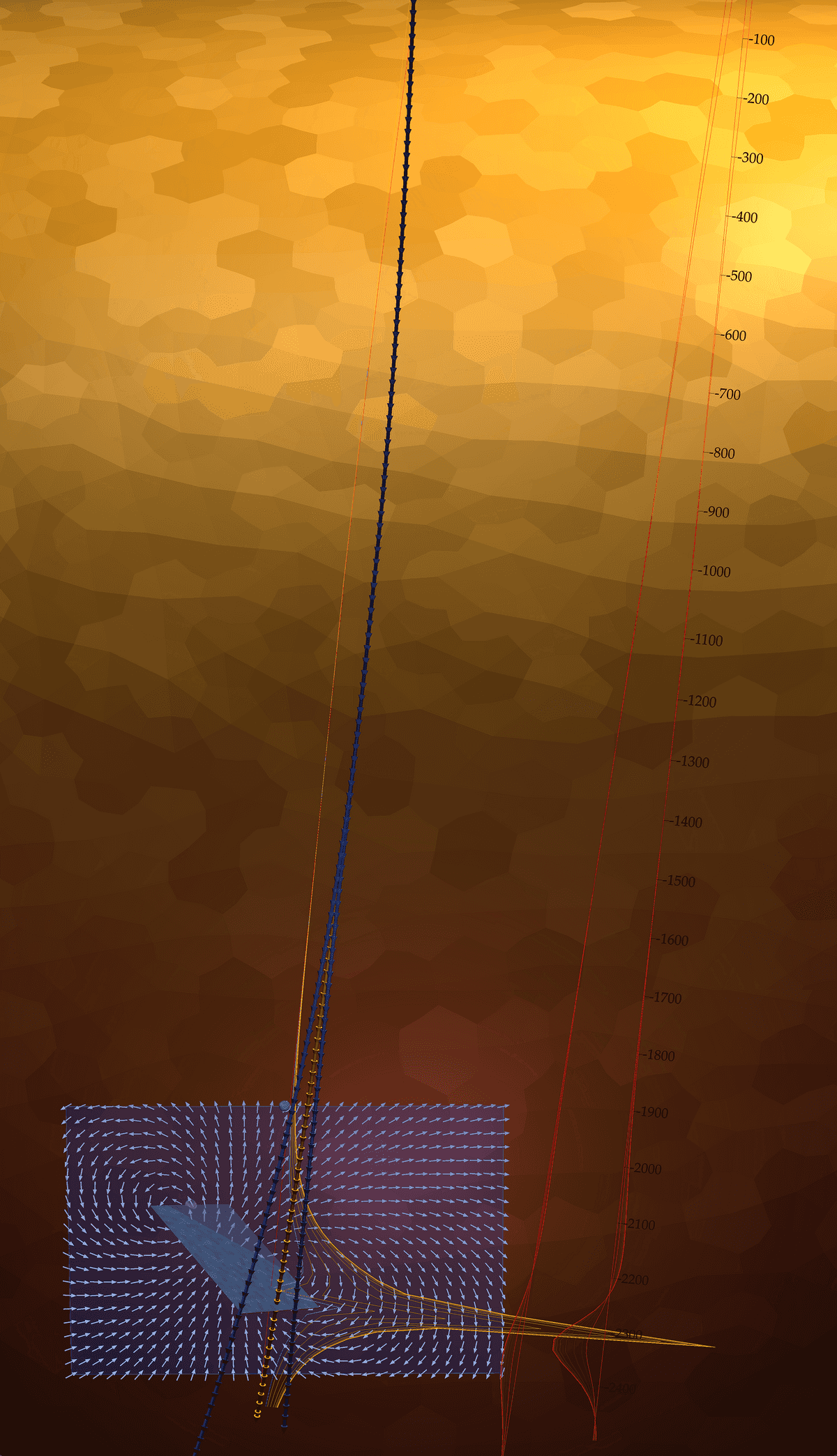
A dipping conductive plate is interseted by a borehole with two near misses. Electromagentic field responses for the intersecting borehole is highlighted in yellow, while the near misses are off to the side in red. Movement of the electromagnetic fields are shown along the surface of a vector plane positioned behind the boreholes.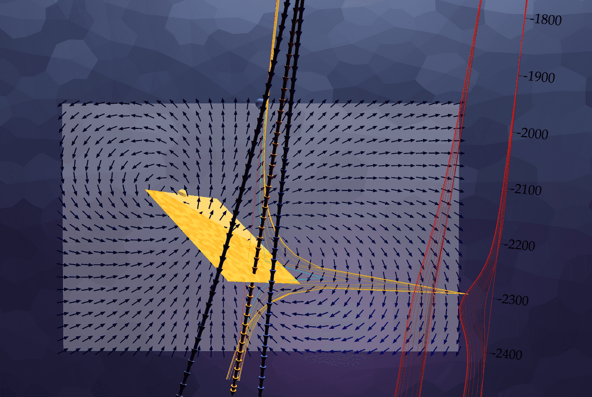
What is Multiloop?
Multiloop is forward modelling software that helps geophysicists visualize electromagnetic responses from conductive meshes. This software is mainly used as a consulting tool that models data collected in the field and compares this to synthetic responses. By carefully noting the differences between data calculated using Multiloop and data collected in the field, a geophysicist can determine the structure of underground conductors, informing drill programs and potentially discovering ore deposits for the mining industry.
Historical Context
Mulitloop was first developed by Yves Lamontagne at Lamontagne Geophysics Ltd. in the 1980's to address the need for better modelling of synthetic conductors in order make sense of the field data collected from time domain electromagnetic geophysics equipment. Multiloop II was later developed as a stand-alone application for Macintosh in the 1990's. It used ribbon conductors to orient thin plates that could approximate the response of potential conductors, and was a powerful consulting tool for the next twenty years.
In the 2000's, work began on Multiloop III, a more powerful modelling software program that uses a hexagonal mesh to calculate the response of curved surfaces and volumes in addition to plates. Originally this was also a stand alone program, however it became cumbersome to have the compute engine and user interface together, and the compute engine was separated from the user interface. An API was created to connect to third party software to query an EM friendly mesh and model the response.
Development of Multiloop GL
As the API was developed, there was a need to create a front end visualizer that could query and test the API. After the initial success of the web-based plotter, a 3D prototype was built to test the feasibility of a web-based visualizer for the Multiloop compute engine. The capable webGL framework three.js was selected to help build the scene and handle orbit controls, and work began on what was to become Multiloop GL.
The first challenge was to create a way in which objects could be moved through the 3D scene. Until this time, objects were somewhat awkwardly positioned by entering values in a dialogue box for coordinate, local offset, strike, dip and plunge of the object, often a frustrating experience when the object moved differently then expected. There needed to be an intuitive interface to move things around.
The answer was inspired by the Douglas Protractor, a tool known to geologists for plotting regional geology. When attached virtually to an object or nearby reference point, any selected object could slide or rotate into position using this protractor. A dialogue box updates the new coordinates, while at the same time providing feedback to allow for fine tuning if required.
A virtual Douglas Protractor allows for any object to be moved and rotated within a 3D scene.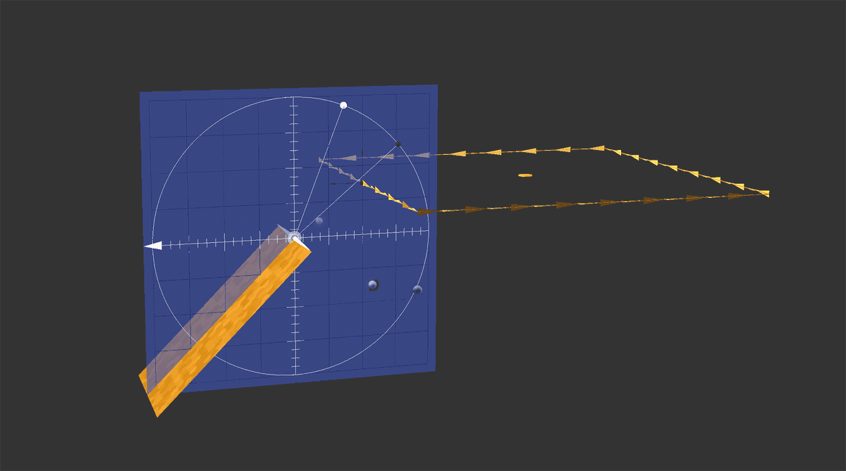
The next challenge was to build an interface to add new meshes using the compute engine, as well as copy, delete and scale existing ones. A shape library was created to store pre-calculated meshes while the interface caught up to the capabilities of the compute engine. Variable conductivity was also a requested feature, and a tool was created to allow conductivity to be "painted" to a shape by dragging a spherical brush through a 3D scene.
A spherical paintbrush tool is used to add variable conductivity to a widened syncline.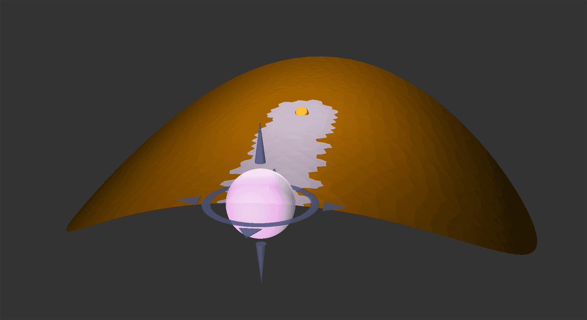
Although plotter allowed for data to be viewed in 2D, part of the Multiloop experience was to visualize data in-situ in the 3D scene. To accomplish this, the Data-Driven Documents library d3.js was used to create x and y axis, and queried to inform proper axis in the 3D scene. The camera position is used to determine which way the labels are facing, and rotates whenever the camera crosses into the next octant, avoiding "mirror image" labelling in the 3D scene.
A vertical electromagenitc response, plotted in 3D for a traverse line calculated by the compute engine.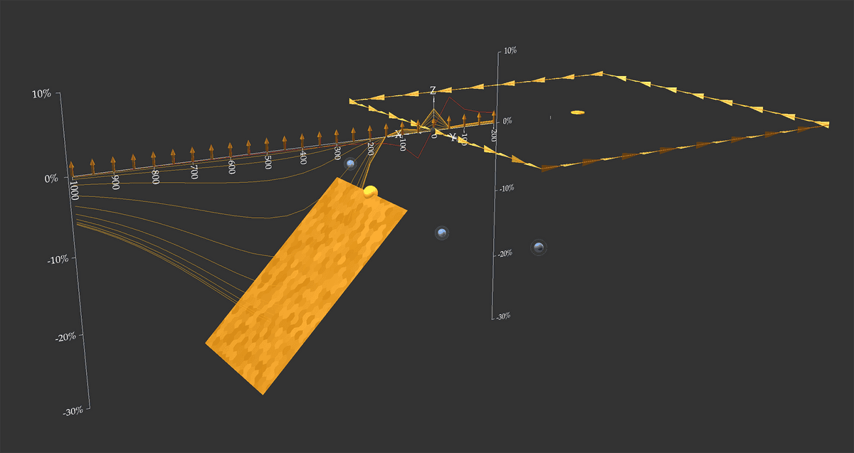
But how did the data get there? At first, a local copy of the compute engine ran on each development machine, and a python server polled a local folder for any new files. It was a sufficient set up for development, but unfeasible to expect a local python server and custom install for every machine that required Multiloop. The solution was to host the compute engine and create a login page that a user could sign into for access. This meant running NGINX and creating a reverse proxy to node.js.
One of the biggest challenges was the file system. It was important to export an entire 3D scene and open the same scene from the exported file. At first, Mulitloop files were simply a collection of numbers in plain text, but the program quickly got to complicated to parse and write without errors. JSON formatted files were adopted to directly string or parse into javascript. A versioning system had to be employed to keep older files from becoming unreadable, but JSON proved to be a very effective and human readable file format. Well almost. Exporting meshes and vector planes with 20 channels of data per vector were quite large, and a binary file system was employed with an accompanying JSON file that described where to find each file needed to re-create the 3D scene.
It was a joy to work on a project with such an ambitious project with such a large arc, and once everything was running, it was a joy to model with.
Multiloop EM Modelling of three 2.5 km boreholes, as presented in Toronto, Canada during Exploration 2017.